How has the urban heat island in my city changed over decades?

An urban heat island is simple: a city is hotter than the countryside around it, because concrete and asphalt soak up sunlight all day and release it slowly at night, while trees and soil cool off fast. Satellites can read the temperature of the ground itself from orbit. That’s the land-surface temperature: how hot the rooftops, roads and fields actually are, not the air. So you can measure how much hotter your city’s surface is than its rural edge, and watch that gap change year after year.

Which data to use, and how

Use this dataset: MODIS Terra LST (short name MOD11A1), a daily map of ground temperature at ~1 km resolution going back to 2000. “LST” means land-surface temperature. It’s the easiest place to start because it has the longest record and one clean number per pixel per day. Later you can add MODIS Aqua LST (MYD11A1), an identical instrument on a second satellite that flies over at a different time of day. That’s handy, because the heat island is usually strongest at night.

Then do four steps (the runnable code further down does all of this; this is just the idea):

1. Pick two boxes. A small latitude/longitude box over your city core, and a matching box over rural land nearby to act as a baseline (a “control”).
2. One number per box per day. Average the surface temperature inside each box. Keep only good-quality pixels (a quality flag marks the trustworthy ones; more on that below).
3. Take the difference. City temperature minus rural temperature. That gap is the heat island, in degrees. Do it separately for day and night.
4. Average over time and fit a trend. Collapse to a yearly average to smooth out cloudy days, then draw the long-term line. Up means the city is pulling away from the countryside, flat means no real change.

That’s the whole method. Below, “How a scientist answers this” names the exact tools, and the Run it cell does it live on synthetic data so you can see each step work.

What you can find out

• Whether the heat-island gap is growing over the years: your city core vs surrounding rural land, all the way back to 2000.
• Day vs night intensity. The gap is usually much bigger at night. Using both MODIS Terra (morning overpass) and MODIS Aqua (afternoon/night) lets you see both.
• Hyper-local hot spots at 70 m, like playgrounds, asphalt parking lots and factory roofs, by switching to ECOSTRESS (ECO2LSTE), a sharper thermal sensor (2018+).
• The urbanization link. Overlay Black Marble (VNP46A2) nighttime city lights and watch the lights (and the heat) spread together.
• Heat and fairness. Overlay the temperature map with demographic data to see which neighborhoods bear the most heat.

What it can’t tell you

• The air temperature people actually feel. The satellite reads the skin temperature of the ground. A sunlit road can be far hotter than the air above it. Surface and air temperature can differ by 5–15 °C. For human heat exposure you must convert it with a model or pair it with weather stations.
• Indoor heat. This is purely an outdoor, top-down view of surfaces. It says nothing about how hot it is inside a building.
• Whether a specific fix worked. You can see a hotspot, but proving that this new park or that cool roof cooled things down needs on-the-ground measurement campaigns, not satellite pixels alone.

Gotchas to watch for

• Surface temperature is not air temperature. This is the big one. LST is how hot the ground is, and it can run 5–15 °C off the air temperature a thermometer reads, so never quote LST as “how hot it felt.” If you need the air value, model the conversion or combine with weather-station data.
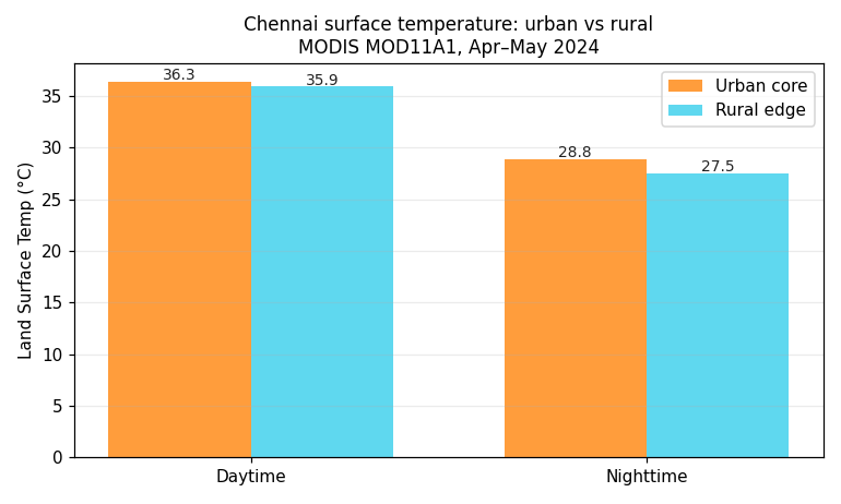
• Clouds wipe out days. A cloudy pixel can’t be measured, so many days drop out, and worse, clouds can leave behind bad values that look reasonable until you average them in. A few of those poisoned pixels are enough to skew your yearly mean. Keep only good pixels using the quality flag (LST_Day_1km_QC, keep QC = 0), then average over a whole year so the clear days fill the gaps.
• Daytime can lie. On a single hot, dry day the city core can look cooler than the parched rural land around it (the “surface urban cool island”), so a one-day daytime check can hand you the opposite of the truth. Lean on night data and average many days instead. The worked example above shows the night gap (+1.3 °C) is ~3× the day gap (+0.4 °C).
• 1 km pixels blur the city edge. At ~1 km, a single pixel can mix city and countryside, smearing the boundary and making the heat island look weaker than it really is. For sharp, modern detail switch to ECOSTRESS (70 m), but note it only goes back to 2018 and visits irregularly, so keep MODIS for the long trend.

The real-data code

The Run it cell above runs this method on synthetic data with no login. Below is the whole recipe against the real archive: search both MODIS LST products, open the HDF-EOS2 granules, mask to good pixels, take the city-minus-rural gap day and night, average over the season, and plot it. It needs a free Earthdata Login.

import earthaccess, numpy as np, xarray as xr
import matplotlib.pyplot as plt

earthaccess.login(strategy="netrc")

# Two boxes: the city core and rural land nearby (the control). This is Chennai, India:
city  = (80.15, 12.95, 80.35, 13.20)   # (W, S, E, N)
rural = (80.45, 12.95, 80.65, 13.20)   # ~25 km east, same latitude band
window = ("2024-04-01", "2024-05-31")  # hot season; widen for the multi-year trend

# 1. Average good-quality LST inside a box from one HDF-EOS2 granule. MOD11A1/MYD11A1
#    are sinusoidal-grid HDF-EOS, so xarray reads them; QC==0 keeps the trusted pixels,
#    and the data are scaled 0.02 K with 0 as fill.
def box_mean(ds, lst_name, qc_name, aoi):
    lst, qc = ds[lst_name], ds[qc_name]
    lon, lat = ds["x"], ds["y"] if "y" in ds else (ds["XDim"], ds["YDim"])
    good = (qc == 0) & (lst > 0)
    sub = lst.where(good & (lon >= aoi[0]) & (lon <= aoi[2])
                         & (lat >= aoi[1]) & (lat <= aoi[3]))
    return float(sub.mean()) * 0.02 - 273.15   # scale to °C

# 2. Walk the daily granules of one product, returning per-day (city, rural) °C.
def daily_gaps(short_name, lst_name, qc_name):
    grans = earthaccess.search_data(short_name=short_name, bounding_box=city,
                                    temporal=window)
    rows = []
    for fh in earthaccess.open(grans):
        ds = xr.open_dataset(fh, engine="rasterio")  # HDF-EOS subdataset reader
        c, r = box_mean(ds, lst_name, qc_name, city), box_mean(ds, lst_name, qc_name, rural)
        if np.isfinite(c) and np.isfinite(r):
            rows.append((c, r))
    return np.array(rows)

day   = daily_gaps("MOD11A1", "LST_Day_1km",   "QC_Day")    # Terra ~10:30 local
night = daily_gaps("MYD11A1", "LST_Night_1km", "QC_Night")  # Aqua  ~01:30 local

# 3. The heat island = city minus rural, averaged over the cloud-free days, day vs night.
uhi_day   = float(np.mean(day[:, 0]   - day[:, 1]))
uhi_night = float(np.mean(night[:, 0] - night[:, 1]))

# 4. Verdict.
print(f"Urban heat island: night {uhi_night:+.1f} °C, day {uhi_day:+.1f} °C "
      f"({len(day)} day / {len(night)} night cloud-free granules)")
print("Night gap >> day gap" if uhi_night > uhi_day else
      "Daytime can read 'cool island' over dry rural land — lean on the night value")

# 5. Plot the two intensities side by side.
plt.bar(["day", "night"], [uhi_day, uhi_night], color=["#f4a261", "#264653"])
plt.axhline(0, c="k", lw=0.8); plt.ylabel("city − rural LST (°C)")
plt.title("Chennai surface urban heat island"); plt.tight_layout(); plt.show()

# Before you trust it: LST is the skin temperature of the ground, not air temperature
# (they differ 5–15 °C) — pair with a weather station to talk about what people actually feel.

Where the data comes from

Everything here comes from NASA through one free login (Earthdata Login). MODIS LST and ECOSTRESS both live at the LP DAAC archive — one DAAC, one set of credentials, so no juggling multiple accounts. Black Marble nighttime lights come from NASA as well.

Sources

• MOD11A1 user guide: https://lpdaac.usgs.gov/products/mod11a1v061/
• ECOSTRESS science: https://ecostress.jpl.nasa.gov/
• Black Marble: https://blackmarble.gsfc.nasa.gov/